My name is Rick.
If I say this statement is not false, is must be true, because not false = true. And yes, I’m Rick.
Another statement:
I’m older than 18.
If I say that statement is not true, it must be false, because not true = false. And again, it works. I’m 17.
Easy, right?
Now, consider this statement:
This statement is false.
We can apply the logic above to draw the following conclusion:
If the statement were true, we would have a contradiction, hence it is not true. Therefore, it must be false.
If the statement were false, we would also have a contradiction, hence it is not false. Therefore, it must be true.
Using the exact same, easy not logic, we get two different answers. This shouldn’t be possible. Because the statement is neither true nor false, we can’t say not true or not false.
But why can we apply that exact same logic to “I’m older than 18”? Perhaps that statement is also not true nor false. We simply don’t know. Maybe I’m $i$ (the imaginary number) years old.
Final question: Does this have anything to do with Schrödinger’s cat thought experiment?
If you know the answer to this mind breaking thought, please let me know.
]]>First, I would like to thank the Nederlandse Filosofie Olympiade for organizing this event, and, above all, mr. Bahorie, my philosophy teacher.
“People say, oh, we need to make ethical AI. What nonsense. Humans still have the monopoly on evil. The problem is not AI. The problem is humans using new technologies to harm other humans.”
―Garry Kasparov. In: Will Knight, Defeated Chess Champ Garry Kasparov Has Made Peace With AI. Wired Magazine, 2020.
In his quote, Garry Kasparov claims we (society) ought not to worry about artificial intelligence (“AI”) because it is solely us who control the evil. In this essay I will argue that hidden in this claim is the exact reason why we should, no, even have to, worry about artificial intelligence.
Upon reading this quote by Kasparov, I immediately remembered one of the most frightening experiences I have had in my own work in AI. A few years ago, I was just starting to learn about AI and decided it would be cool if I could make a robot that automatically figured out what the quickest path through a maze would be. I quickly wrote a maze app and then built a self-learning AI (which should not be considered sophisticated in any way). I let the AI do its thing and after just a couple of seconds, astonishing results presented themselves–the robot could solve the maze in just a handful of moves while the theoretical limit should be at least in the hundreds. Upon investigation, I discovered my maze code had a critical bug, allowing the robot to skip parts of the grid entirely. This was scary: I had written the maze code as well as the AI from scratch myself and the AI found a bug in just a couple of seconds. In a sense, my own AI became smarter than me. Of course, this project was just an experiment and real world systems are more well-tested, right? Someone who thinks about ‘well-tested’ misses the point: AI–especially much more sophisticated AIs than mine, like the one that defeated Kasparov at chess–can do things it was not explicitly programmed to do, and worse, it might even do things its creators did not even imagine.
I will start by giving a bird’s eye view of the field of artificial intelligence. Then I will explain how it follows that AI is unlike any technology humanity has ever seen. Next, I will move on to discuss Aristotle’s and Kant’s view on ethics. Finally, I will conclude by applying their philosophies to Kasparov’s claim and AI in general to show how AI is, in fact, a threat to humanity.
In this section, I will give a quick overview of artificial intelligence and highlight some concepts I think are of importance in this essay.
There are two main approaches to AI: expert systems and learning systems. Expert systems are huge databases containing thousands of human-defined rules and facts. A search algorithm combines these facts and rules into what would be the best answer to a question, where ‘best’ is, again, based on a set of human-defined criteria. It should be intuitive that these systems will never outperform human intellect.
Personally, I would argue only so-called “learning systems” can be considered “artificially intelligent.” Such a system makes an observation about the world, takes an action, and observes the results of that action. Based on whether the results are in correspondence with some predefined ‘objective’, the AI knows whether the underlying action was “good” or “bad” and updates its systems accordingly, getting better continuously1. In other words, the concept of “machine learning” can be understood as a computer optimizing some ‘objective.’ Finally, learning systems have two interesting properties: 1) theoretically they can get infinitely–most definitely superhuman–good at any particular task (where a task can be quite complex like “drive a car” or “write a book”) and 2) humans have no way to interpret the way these systems reach conclusions 2.
For the rest of this essay, I will use “AI” to refer specifically to the learning systems.
I will make a quick note on AI versus other kinds of technology. While it is true that technology has been very destructive when used as a weapon, just the Manhattan Project alone speaks volumes, AI is fundamentally different. Where every weapon up until this point has required human supervision, or at least its use required human initiation, AI can operate independently. Furthermore, because learning systems can quickly outlearn humans, it is impossible for us to even understand AI the way we understand everything else we build.
In this section I will clarify the positions of Kant and Aristotle and how their philosophies demonstrate ethics are unique to humankind.
Aristotle talks about ethics in terms of “arete”, or virtues–certain positive qualities, or traits, which can be considered the driving force behind “good” actions. A virtuous person is led by their virtues, hence making the “right” choices and doing “good” things, as their actions are in harmony with the virtues. This philosophy assumes the idea of humans as animale rationale, rational animals, who can make rational decisions about whether an action is good or bad judging by the relevant virtues. Animals lack these virtues and can therefore be good nor evil.
Immanuel Kant argued that the only unquestionably good virtue is what he calls the “good will”, because other virtues could be misused to do bad things. After all, what good is loyalty if one is loyal to a bad king? According to Kant, actions stemming from the good will are considered to be “good.” Humans, then, should use ‘reason’ to determine whether their actions correspond with the good will to determine whether or not they are morally right. This is possible because where animals act based on instincts, humans actions stem from reason, referring to the animale rationale again. Kant noticed that different motivations, maybe even just pure randomness, might lead to the exact same outcome as actions that were carefully examined. While they should be appreciated, Kant says they are not necessarily “good” actions because they have no foundation in the good will. It then follows that unlike humans, animals, which act solely based on their instincts and they lack reason, cannot reason about the ethics of their actions nor be held responsible for them.
Aristotle’s and Kant’s ethics reveal some interesting truths about the claims and their underlying assumptions in Kaspraov’s claim, which I will discuss next.
Just like animals, which act solely based on their innate instincts, artificially intelligent computers lack reason as well as virtues. Consequently, according to both Aristotle and Kant, it is impossible for a computer to “do the right thing”, by definition. This proves Kasparov’s claim that “humans still have the monopoly on evil”, as they are the only ones capable of doing evil things in the first place. In fact, humanity’s monopoly on evil is perpetual. Before that, Kasparov said: “People say, oh, we need to make ethical AI. What nonsense,” which, as I have proved, is not just nonsense, but actually fundamentally impossible.
The problem lies in the second part of the quote: “The problem is not AI. The problem is humans using new technologies to harm other humans.” While historically speaking new technology is extremely likely to be used for evil purposes, it is not our main issue in the case of AI. As I have personally experienced in my little maze experiment, AI can do things its creator did not intend, and cannot even imagine. Hence, subscribing to the idea that “the problem is humans using …” seems morally wrong to me. Moreover, the complete lack of a ‘safety net’ combined with the extraordinary power AI possesses is where the danger lies. We should not worry about AI because it might turn evil; we should worry about AI exactly because it cannot turn evil as evil is a concept of ethics and thus a human construct. A machine has no morale; it lacks what I call ethical intelligence. It does not reason about what is good and what is bad. It just “does”.
We will be playing a game of ‘Russian Roulette’ at an unfathomably large scale. One accidentally ill-defined ‘objective’ could lead an AI to decide humanity is an obstacle in its mission and it better be annihilated. AI’s ‘good’ (meaning corresponding with its ‘objective’) is completely different from human ‘good’ (which is based on human qualities).
To summarize, I have explained how computers can use machine learning to teach themselves how to be intelligent and how AI is fundamentally different from all technology humanity has ever seen, because of its relative autonomy and unpredictability. After that, I demonstrated how the virtue ethics of Aristotle and Kant’s philosophy of reason and a good will prove ethics is something intrinsically human. From there, it follows that Kasparov was right in saying “humans still have the monopoly on evil”. However, in my opinion Kasparov was too naive in assuming AI needs ethics to be destructive, and it is its inherent lack of ethics that make an AI even more dangerous.
An interesting question remains. Imagine we train an AI to mirror human decision making3. After learning and improving on itself for a long time, let’s say it is impossible for anyone to tell the difference between this system and a real human (in other words, it passes the “Turing Test”). Should we consider it human? Virtue ethics tells us the answer is ‘no’ because this AI lacks virtues and thus proper motivation behind its actions. Kant would say we should appreciate this human-like computer, but its actions can still not be considered “good.” Personally, however, I think this case requires further investigation because if we were to trace back the actions of the AI to where it learnt them, we will eventually end up with a real human, and with them their virtues. These virtues are, in a way, what inspired the AI to do what it did, and so it could be argued that the AI is, interestingly enough, still acting on human virtues. Here is the dilemma: is a human responsible, or the AI? The former seems evil, the latter impossible.
1 I should note that “good” and “bad” in this context refer to the ‘objective’ and explicitly not ethics in any way.
2 For the purpose of conciseness, I will not explain why this is true. Human interoperability is an active area of research beyond the scope of this essay.
3 Assuming this is possible.
]]>You can download the source code on my GitHub.
]]>Not having strict supervision allows for easy cheating. No one will know if you use a dictionary. No one will know if you use a calculator. And no one will know if you collaborate with your peers. This got me thinking. If my bedroom is my workplace and I can cheat so easily, does this mean I get a free ride to being a billionaire?
I don’t believe that is the case. Why not? I have come to the conclusion that cheating at school is nothing like cheating in real life. In fact, this “cheating” thing is actually appreciated by employers. Employers don’t care if you use a calculator or dictionary. Using all available tools to the fullest extent is a positive skill. Furthermore, employers value employees who collaborate and discuss difficult problems with other people.
At school, however, you will likely be disqualified for doing any of those things during a test. Weird, since I’m at school to prepare for my life. And my life just happens to provide all of those tools1.
Why do children spend countless hours doing basic arithmetic, when they will be using a calculator for all serious decisions after they graduate? Seriously, who is going to do taxes from the top of their head when they can easily use a calculator? I’m not advocating to stop teaching children math. On the contrary, I actually do think teaching students why addition exists, what it is and when they should use it are important topics that everyone should know. But I don’t care if they can add up 90234 and 87623 leaving a calculator (phone) in their pocket.
I’m also not advocating to stop teaching languages at school and relying on dictionaries instead. I wouldn’t have been able to write this text if I didn’t know English. But I also believe a dictionary helped me improve this text. It’s a combination of practice and resources that made this text what it is. I’m sure native speakers will find some mistakes, and I would love to know how to improve this text but at least we learned Shakespeare died in 1616.
Everyone has access to almost all of mankind’s knowledge regardless of where they are thanks to websites like Wikipedia. That’s a wonderful thing. This is no excuse, however, to stop education altogether; or humans would have been replaced already. Knowing how to apply something requires context, analytical skills and creativity, things a computer cannot yet do, but we can teach children.
Many people say you only fool yourself by cheating. I agree. Cheating is bad if it will hurt you later on. I don’t believe collaborating will ever hurt me. Nor do I believe using a dictionary will.
“But knowing something is quicker than looking it up.” Absolutely! I wish I knew how to provide first aid in pressing situations. I wish I hadn’t wasted time learning to memorize facts I don’t use. And in the rare event of me needing to know who painted some piece, I have Wikipedia right in my pocket.
It’s not fair to cheat at an exam and earn a certificate tricking people into believing you can do something in isolation, when in fact you cannot. So will I study for that exam? Probably not, but I will make sure I can get things done.
Surprisingly, exercises are that impossible to cheat at are, besides the fairest, possibly among the best exercises we can spend time on. Filling out a fancy survey, read exam, may be a way to validate the products in an assembly line, but one would be stupid to believe human qualities can be captured by a number. We shouldn’t test humans the same way we test tools. But most importantly, we are only teaching students facts we know today, and that does not seem to be particularly responsible in a world evolving this rapidly.
An alternative to exams could be asking students to devise something new. After all, how could one cheat at doing something that does not exist yet? Writing a philosophical essay, debating issues in society or writing computer programs seem good places to start. Students should be free to use the tools that are available to professionals in the field, work within common constraints such as deadlines, and above all, be able to collaborate. Using a smart rotation system it would still be possible to extract individual student performance from a shared environment.
Exercises I can cheat at are exercises, for what exactly? I think school should pose exercises I can’t cheat at. If cheating takes time that could be made as a constraint on the exercise. Looking up how to make an argument during a debate won’t sound very convincing. Math requires exact answers and computers often can’t manage that. Fair enough, we will have to do it by hand. There is nothing inherently bad about it.
If I can cheat at something and still get the correct answer or get a project done, I have found a loophole in education. It means education is not prepared for the technological advancements. School today doesn’t really prepare us for the future. Let’s change that.
I am aware of the fact that due to their insane success, many tutorials have been written about neural networks. Many try to impress you by giving a vague proof of backpropagation. Others will confuse you with explanations of biological neurons. This post is not yet another copy of that, nor will I be ignoring the mathematical foundations (which is contrary to the goal of this series). In this post I hope to give you an understanding of what a neural network actually is, and how they learn.
Here is the corresponding notebook where you can find a complete and dynamic implementation of backprop (see later) for any number of layers.
As I just mentioned, in this post we will classify handwritten digits. To do so, the MNIST dataset [1]. It consists of 60000 28 by 28 grayscale images like the following:
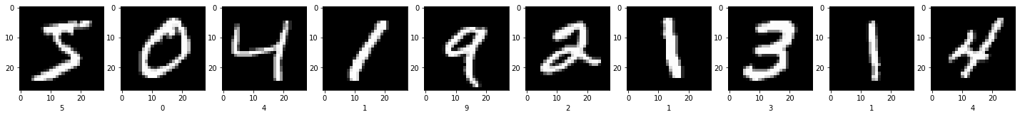
In computer vision, a subfield-ish of machine learning, each pixel represents a feature. The images in MNIST are grayscale so we can use the raw value of the pixels. But other datasets might be in RGB format and if that’s the case each channel of a pixel will be a feature.
It turns out that the classifiers we have seen thus far are not capable of classifying data with this many features ($28 \times 28 = 784$). For instance, the 4’s in the images above are quite different, most certainly when represented as a matrix.
This does not mean the problem cannot be solved. In fact, it is solved. To understand how, let’s learn about neural networks.
Think about a classification as follows
where $x$ is an input vector, being mapped to a prediction vector $\hat{y}$.
If you were to visualize the individual elements of both vectors, you would get something like this:
Let’s look at the definition of the hypothesis function $h$ again: (see softmax regression):
\[h_\theta(x) = \sigma(X \cdot \theta) = \begin{bmatrix}p(y = 0 | x; \theta) \\ p(y = 1 | x; \theta) \\ p(y = 2 | x; \theta)\end{bmatrix} = \begin{bmatrix} \frac{\exp(\theta_0^Tx)}{\sum_{j=1}^k \exp(\theta_j^Tx)} \\ \frac{\exp(\theta_1^Tx)}{\sum_{j=1}^k \exp(\theta_j^Tx)} \\ \frac{\exp(\theta_2^Tx)}{\sum_{j=1}^k \exp(\theta_j^Tx)} \end{bmatrix}\]The most important thing to understand is that every feature $x_j$ is multiplied by a row $j$ in $\theta$ ($\theta_j$); each feature $x_j$ impacts the probability of the entire input $x$ belonging to a class. If we visualized the “impacts” in the schema, we would get this:
One thing this graph does not account for is the bias factor. Let’s add that next:
The network seems, on a high level, very representative of the underlying math. Please make sure you fully understand it before moving on.
Let’s now look at an individual node in this network.
The node for $\hat{y}_1$ multiplies the inputs $x_j$ by their respective parameters $\theta_j$ and, because we are dealing with vector multiplication, adds up the results. In most cases, an activation function is then applied.
\[\hat{y}_1 = g\left(\displaystyle\sum_{j=0}^n \theta_j \cdot x_j\right)\]This is the exact model we discussed in the logistic regression post.
In the context of a classifier network, people call nodes such as $\hat{y}$ “neurons.” The complete network is, therefore, considered a “neural network.” For the sake of consistency I will also use those terms, but I will simply define “neuron” as “node.” Keep in mind that the biological definition of neuron is something else entirely.
Simple networks like these, it’s just a logistic classifier represented as a network, fail at large classification tasks because they have too few parameters. The entire model is too simple and it will never be able to learn from more interesting datasets such as MNIST. However, logistic regression can still be used in this problem. In fact, the main intuition I will present in this post is that a neural network is just a chain of logistic classifiers.
The graph I presented before can be modified to include another layer, or multiple other layers, the so-called “hidden layers.” These layers are placed between the original input and the original output layer. The reason they are called “hidden” is because we do not directly use their values; they simply exist to forward the weights through the network. Note that these layers also have a bias factor.
Because the hidden layer (blue) is not directly related to the number of features (the input layer, in red) or the number of classes (output layer, in green) they can have an arbitrary number of neurons, and a neural network can have an arbitrary number of layers (denoted $L$).
This schema looks promising, but how does it really work?
Let’s start by looking at how we represent the weights. In the first two posts (polynomial regression and logistic regression) the weights were stored in a vector $\theta \in \mathbb{R}^n$. With softmax regression we started using a matrix $\theta \in \mathbb{R}^{n \times K}$ because we wanted an output vector instead of a scalar.
Neural networks use a list to store weights, often denoted as $\Theta$ (capital $\theta$), each item $\Theta^{(l)}$ being a weight matrix. Unlike the schematic, the shapes of the hidden layers often change throughout the network, so storing them in a matrix would be inconvenient. Each weight matrix has a corresponding input and output layer. A particular weight matrix, in layer $l$, is $\Theta^{(l)} \in \mathbb{R}^{(\text{number of input nodes} + 1)\atop \times \text{number of output nodes}}$.
A Python function initializing the weights for a neural network:
# inspired by:
# https://github.com/google/jax/blob/master/examples/mnist_classifier_fromscratch.py
def init_random_params(layer_sizes, rng=npr.RandomState(0)):
return [rng.randn(nodes_in + 1, nodes_out) * np.sqrt(2 / (nodes_in + nodes_out))
for nodes_in, nodes_out, in zip(layer_sizes[:-1], layer_sizes[1:])]
This function takes a parameter layer_sizes
, which is a list of the number of nodes in each layer. For this problem I build a neural network with 2 hidden layers, each with 500 neurons. Note that the number of nodes in the input and output layer are determined by the dataset.
weights = init_random_params([784, 500, 500, 10])
init_random_params
automatically accounts for a bias factor, so we get the following shapes:
>>> [x.shape for x in weights]
[(785, 500), (501, 500), (501, 10)]
To compute the predictions, given the input features, we use a (very simple) algorithm “feedforward.” We loop over each layer, add a bias factor, compute the output by multiplying by the corresponding weight matrix, and finally apply the activation function.
It’s easier in Python:
def forward(weights, inputs):
x = inputs
# loop over layers
for w in weights:
x = add_bias(x)
x = x @ w
x = g(x)
return x
Given the list of weights $\Theta$, we know that given the input $x = a^{(1)}$, the activations in layer 2 should be $a^{(2)} = g(x \cdot \Theta^{(2)})$. The activations in layer 3 should be $g(a^{(2)} \cdot \Theta^{(3)})$. Generally, the activation in layer $l$ is $g(a^{(l-1)} \cdot \Theta^{(l)})$. Note that the above code example uses x
as the only variable name for convenience, but that does not necessarily mean $x$ as in input.
In short, $h_\theta(x)$ can take on other forms than a matrix multiplication.
Next, let’s discuss how to train a neural network. People often think this is a very complicated process. If that’s you, forget everything you’ve learnt so far because it’s actually quite intuitive.
Once you realize that the values for any $\Theta$ yield deterministic activations in the entire neural network given some input, it is understandable that not every activation in a hidden layer is desired, even though they are not directly interpreted (in fact, interpreting the values of hidden layers is an active problem). This implies that in order to have good predictions, we also need good activations in hidden layers.
We would like to compute how we need to change each value of $\Theta$ so that we get the correct activations in the output layer. By doing that, we also change the values in the hidden layers. This means that the hidden layers also carry an error term (denoted $\delta^{(l)}$), while that’s not directly obvious if you only think about the final output layer. The same thing in reverse: by inspecting the error in each hidden layer, we can compute the change (gradient) for the weight matrices.
The only layer for which we immediately know the error term is the output layer. Because it serves as a prediction layer we can compare its output to the labels. The error for layer $L$ is given as
\[\delta^{(L)} = \hat{y} - y\]For all previous layers we can compute the error term with the following formula:
\[\delta^{(l)} = ((\Theta^{(l)})^T \delta^{(l+1)})\ .* g'(a^{(l)})\]Because $\delta^{(l)}$ is depended on $\delta^{(l+1)}$ the error terms must computed in reverse other. It is also dependent on $a^{(l)}$, the activations of layer $l$, so in order to compute it we first need to know the exact activation in this layer. That’s the reason a full forward propagation is usually computed before starting backpropagation, saving activations along the way.
x = inputs
activations = [inputs]
for w in weights:
x = add_bias(x)
x = x @ w
activations.append(x)
x = g(x)
predictions = x
Now to compute the error term, we start by computing the error in the final layer. The error is transposed to match the format of the other errors we will compute.
final_error = (predictions - y).T
errors = [final_error]
We will compute the other errors in a loop. A few things to note:
We index our activations by [1:-1]
so we skip the first layer (the input has no error term) and the output layer (we already have computed that).
We skip the first node in each layer; it is defined as 1.
Finally, weights[-(i+1)]
is the weight matrix indexed from the back (-1
because i
starts at 0).
These things are important things to keep in mind when doing backprop, but in this context it’s easy to understand.
for i, act in enumerate(activations[1:-1]):
# ignore the first weight because we don't adjust the bias
error = weights[-(i+1)][1:, :] @ errors[i] * g_(act).T
errors.append(error)
This snippet uses the derivative of sigmoid g_
. It is defined as:
def g_(z):
""" derivative sigmoid """
return g(z) * (1 - g(z))
or
\[\frac{d}{dz} g(z) = g(z) \cdot (1 - g(z))\]Finally, we flip the errors so they are arranged like the layers:
errors = reverse(errors)
For the sake of completeness:
def reverse(l):
return l[::-1]
Recall that a gradient is a multidimensional step for a weight matrix to decrease the error.
We now know the error for each layer. If we go back to logistic regression, the building block of neural networks, you can think of these as the loss of each layer. This means that we can use the same equation we developed in a previous post to compute the gradient for each weight matrix corresponding to each error term. Except the loss is now $\delta^{(l + 1)}$ and the input $a^{(l)}$.
\[\Delta^{(l)} = \frac{1}{m} \cdot \delta^{(l + 1)} a^{(l)}\]grads = []
for i in range(len(errors)):
grad = (errors[i] @ add_bias(activations[i])) * (1 / len(y))
grads.append(grad)
Congratulations! You now know backpropagation. Fun note: because we are learning multiple layers, we are doing deep learning. Just so you know.
The way backpropagation is usually taught is by presenting it as a method for finding the derivative for the cost function. A great intuition on backpropagation from that perspective is written by Andrej Karpathy in his Stanford course. I’ll let him explain it himself.
Because the entire dataset consists of $60000 \cdot 28 \cdot 28 \approx 4.7 \cdot10^7$ elements, it’s too big for most computers to fit in the RAM at once. That’s the reason we use “batching”, loading only a few (100 in this case) at a time.
lr = 0.001
for epoch in range(2):
print('Starting epoch', epoch + 1)
for i in range(len(x_train)):
inputs = x_train[i][np.newaxis, :]
if x_train[i].max() > 1: print('huhh', i, x_train[i].max())
labels = T([y_train[i]], K=10)
grads = backward(inputs, labels, weights)
for j in range(len(weights)):
weights[j] -= lr * grads[j].T
if i % 5000 == 0: print(stats(weights))
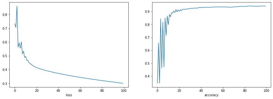
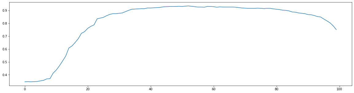
This should get you an accuracy of $90\%$.*
For the complete code, refer to the notebook.
You might be wondering if you need to implement everything we did today when you are building a neural network. Fortunately, that’s not the case. Many deep learning libraries exist, PyTorch and TensorFlow + Keras being the most popular.
While this series focusses on the fundamentals, I would like to show you an example in Keras because it’s the easiest, in my opinion. (you should be able to find other tutorials on MNIST in all other frameworks easily if you’re into that)
You can define a model as just a list of tf.keras.layers
objects, and Keras will automatically initialize the weights.
model = tf.keras.Sequential([
tf.keras.layers.Dense(500,
activation='sigmoid',
input_shape=(28 * 28,)),
tf.keras.layers.Dense(500, activation='sigmoid'),
tf.keras.layers.Dense(10, activation='sigmoid')
])
*This model does not have the same accuracy some other models do because I skipped some things to keep the post concise. In a future post I will present those techniques.
Apart from the ability to stack logistic classifiers, another thing that makes neural networks powerful is that we can combine different kind of layers. Today we have looked at “dense” layers, layers consisting of a matrix multiplication and activation function. Convolutional and dropout layers, for example, are other type of interesting layers I will cover in a future post.
In the next post I will cover optimization algorithms so we can train larger neural networks much faster.
You should check out the TensorFlow Playground, a website where you can play around with neural networks in a very visual way to get an even better intuition for how feedforward works.
I added [2] as a reference to learn more about backpropagation as a technique to differentiate the loss function for neural networks.
[1] LeCun, Y., Cortes, C., & Burges, C. (2010). MNIST handwritten digit databaseATT Labs [Online]. Available: http://yann. lecun. com/exdb/mnist, 2.
[2] Atilim Gunes Baydin and Barak A. Pearlmutter and Alexey Andreyevich Radul (2015). Automatic differentiation in machine learning: a surveyCoRR, http://arxiv.org/abs/1502.05767.
]]>Recall from the previous post that classification is discrete regression. The target $y^{(i)}$ can take on values from a discrete and finite set. In binary classification we only considered sets of size $2$, but classification can be extended beyond that. Let’s look at the complete picture where $y^{(i)} \in {0, 1, \ldots K}$.
The model we build for logistic regression could be intuitively understood by looking at the decision boundary. By forcing the model to predict values as distant from the decision boundary as possible through the logistic loss function, we were able to build theoretically very stable models. The model outputted probabilities for each instance belonging to the positive class.
However, in multiclass classification it’s hard to think about a decision boundary splitting the feature space in more than 2 parts. In fact, such a plane does not even exist. Furthermore, the log loss function does not work with more than two classes because it depends on the fact that if an instance belongs to one class, it does not belong to the other. So we need something else.
Let’s look at where we are thus far. A schematic of polynomial regression:
A corresponding diagram for logistic regression:
In this post we will build another model, which is very similar to logistic regression. The key difference in the hypothesis function is that we use $\sigma$ instead of sigmoid, $g$:
As I just mentioned, we can’t measure distances over a single “class dimension” (by which I mean the probability of an instance belonging to the positive class). Instead, for multiclass classification we think about each class as a separate channel, or dimension if you will. All of these channels are accumulated in an output vector, $\hat{y} \in \mathbb{R}^K$.
Let’s take a look at what such a vector would look like. For convenience, we define a function $T(y): \mathbb{R} \rightarrow \mathbb{R}^K$ which maps labels from their integer representation (in $0, 1, \ldots k$) to a one hot encoded representation. This function takes into account the total number of classes, $3$ in this case.
\[T(0) = \begin{bmatrix}1 \\ 0 \\ 0 \end{bmatrix} \quad T(1) = \begin{bmatrix}0 \\ 1 \\ 0 \end{bmatrix}\]The instance in class $0$ has a $100\%$ chance of belonging to $1$, and a $0\%$ chance for all other classes. We would like $h$ to yield similar values.
In Python $T$ could be implemented as follows:
def T(y, K):
""" one hot encoding """
one_hot = np.zeros((len(y), K))
one_hot[np.arange(len(y)), y] = 1
return one_hot
If you don’t yet see why this would be useful yet, hang on.
Up until now $x \cdot \theta$ has always had a scalar output, an output in one dimension. However, in this case the resulting value will be a vector where each row corresponds to a certain class, as we have just seen. While this could be achieved by initializing $\theta$ as an $n \times K$ dimensional matrix, which we will also do, the dot product would be of little meaning.
That’s the reason we define another activation function, $\sigma$. As you may remember from last post, $g$ is the general symbol for activation functions. But as you will learn in the neural networks post (stay tuned) the softmax activation function is a bit of an outlier compared to the other ones. So we use $\sigma$.
For $z\in\mathbb{R}^k$, $\sigma$ is defined as
\[\sigma(z) = \frac{\exp(z_i)}{\sum_{j=1}^k \exp(z_j)}\]which gives
\[p(y = i | x; \theta) = \frac{\exp(\theta_j^Tx)}{\sum_{j=1}^k \exp(\theta_j^Tx)}\]where $\theta_j \in \mathbb{R}^m$ is the vector of weights corresponding to class $i$. $p$ is the probability. For more details on why that is, refer to this document, section 9.3.
The hypothesis function $h$ yields a vector $\hat{y}$ where each row is the probability of the input $x$ belonging to a class. For $K = 3$ we have
\[h_\theta(x) = \sigma(X \cdot \theta) = \begin{bmatrix}p(y = 0 | x; \theta) \\ p(y = 1 | x; \theta) \\ p(y = 2 | x; \theta)\end{bmatrix} = \begin{bmatrix} \frac{\exp(\theta_0^Tx)}{\sum_{j=1}^k \exp(\theta_j^Tx)} \\ \frac{\exp(\theta_1^Tx)}{\sum_{j=1}^k \exp(\theta_j^Tx)} \\ \frac{\exp(\theta_2^Tx)}{\sum_{j=1}^k \exp(\theta_j^Tx)} \end{bmatrix}\]See how $T$ fits into the picture?
To get a final class prediction, we don’t check if the number exceeds a certain threshold ($0.5$ in the last post), but we take the channel with the highest probability. In mathematical terms:
\[\text{class} = \arg\max \hat{y}\]One thing I would like to point out here is that
\[\displaystyle\sum_{j=1}^k h_\theta(x)_j = 1\]This is obvious because the sum of numerators in $h$ is equal to the denominator, by definition.Intuitively, the model is $100\%$ sure each instance belongs to one of the predefined classes. Furthermore, because $\exp$ is, of course, an exponential function, large elements in $\theta^Tx$ will be “intensified” by $\sigma$ to get a higher probability, also relatively speaking.
A vectorized python implementation:
def softmax(z):
return np.exp(z) / np.sum(np.exp(z))
When implementing softmax, $\sum_{j=1}^k \exp(\theta_j^Tx)$ may be very high which leads to numerically unstable programs. To avoid this problem, we normalize each value $\theta_j^Tx$ by subtracting the largest value.
The implementation now becomes
def softmax(z):
z -= np.max(z)
return np.exp(z) / np.sum(np.exp(z))
This normalization step has no further impact on the outcomes.
For the sake of completeness, here is the final implementation for the hypothesis function:
def h(X, theta):
return softmax(X @ theta)
The loss function is used to measure how bad our model is. Thus far, that meant the distance of a prediction to the target value because we have only looked at 1-dimensional output spaces. In multidimensional output spaces, we need another way to measure badness.
Negative log likelihood is yet another loss function suitable for these kinds of measurements. It is defined as:
\[J(\theta) = -\displaystyle\sum_{i = 1}^m \log p(y^{(i)}|x^{(i)};\theta)\]When I first encountered this function it was extremely confusing to me. But it turns out that the idea behind it is actually brilliant and even intuitive.
Let’s first look at the plot of the negative log likelihood for some arbitrary probabilities.
As the probability increases, the loss decreases. And because we only take the negative log likelihood of the current class, $y^{(i)}$ in the formula, into account, this looks like a nice property. Moreover, when we maximize the probability for the correct class, we automatically decrease the probabilities for other classes because the sum is always equal to $1$. This is an implicit side effect which might not be obvious at first.
We always want to get the loss as low as possible. The negative log likelihood is multiplied by $-1$, which means that you could also look at it as maximizing the log likelihood:
\[\displaystyle\sum_{i = 1}^m \log p(y^{(i)}|x^{(i)};\theta)\]Because all machine learning optimizers are designed for minimization instead of maximization, we use negative log likelihood instead of just the log likelihood.
Finally, here is a vectorized Python implementation:
def J(preds, y):
return np.sum(- np.log(preds[np.arange(m), y]))
preds[np.arange(m), y]
indixes all values of preds
for each class of y
, discarding the other probabilities.
If you would like to play around with the concepts I introduced yourself, I recommend you check out the corresponding notebook.
You now have all the necessary knowledge to learn about neural networks, the topic of next week’s post.
]]>It’s well-known that projects without documentation don’t get the attention they deserve. And rightfully so, because it’s very hard for new “users” (developers who consume your package) to get started with your project if documentation is lacking. However, writing and maintaining documentation is often seen as a boring task. Besides, your documentation will quickly be outdated if you don’t update it.
Luckily, great tools exist to generate documentation for you. In this post, I’d like to give you a quick introduction to jazzy
: a Realm project to automatically generate great documentation pages for your project. And it even works with Objective-C.
We’ll also look at how to host the generated documentation on GitHub Pages, for free! Simply put, a deployed version of your documentation is much better than just sending your users some HTML files.
And as icing on the cake, you’ll also learn how to use GitHub Actions to generate new docs each time you deploy a new version of your package, format your code through SwiftLint, and run your tests. All automated and completely free!
]]>In the previous post I explained polynomial regression problems based on a task to predict the salary of a person given certain aspects of that person. I also discussed basic machine learning terminology. In this post I describe logistic regression and classification problems. By working through another example, predicting breast cancer, you will learn how to build your own classification model. I will also cover alternative metrics for measuring the accuracy of a machine learning model.
%pylab inline
The code is available in the corresponding GitHub repository for this series (leave a star :)). I encourage you to run the notebook alongside this post.
In a classification problem, the target values are called labels. Each label corresponds to a certain class such as “car”, “blue” or “malignant.” Each instance belongs to a certain class*, thus having a label. Both the labels and classes have to be unique, but more than one instance per class is allowed—it’s actually strongly encouraged. Usually each class’ label has an integer value starting at 0 and following classes get a label of 1, 2, 3, etc. This gives us the property that \(y^{(i)} \in \{0, 1, \ldots, K \}\) where $K$ is the number of classes.
With the terminology of the previous post, we could state that for binary classification \(y \in \{0, 1\}^m\) where \(0\) and \(1\) are labels. Further, in binary classification the instances belonging to the $0$-class are the “negatives”, often indicating the absence of a something, and $1$ are the “positives”. Another way to look at this is that for negatives there is a $0\%$ chance of something occurring where for positives there’s a $100\%$ chance. These percentages will, hopefully, be the output of a logistic regression model.
*If you wish to classify instances as not belonging to a certain class, you assign a “not classified” class.
The dataset we are working with today is the Breast Cancer Data Set [1]. For this dataset we have the following properties:
\[m = 669 \quad \quad n = 9\]To keep the blog post concise and focussed I added explanations in the notebook explaining how to load and clean the data with pandas.
Much like the previous problem we need a way to map input values to output values. We will once again call this model \(h_\theta\).
Remember the model from polynomial regression:
\[h_\theta(x) = \theta^Tx\]We will make one small change to this model to work with classification.
Note that the model can output values much greater than $1$ and much smaller than $0$. This is unnatural and not desired—we would like to get values between $0$ and $1$ so we can interpret the output as probabilities. To achieve this we use the sigmoid function:
\[g(z) = \frac {1}{1+e^{-z}}\]Note: $g$ is a symbol for an activation function (more on that in future posts), not sigmoid.
While this function looks complicated, it’s easy to see why it’s used when you look at its graph:
For values $x < 0$ we have that $g(x) < 0.5$ and for $x < 0$ we have $g(x) > 0.5$.
In Python you can just copy the formula over:
def g(z):
""" sigmoid """
return 1 / (1 + np.exp(-z))
As you can see, if we modify $h$ to be
\[h_\theta(x) = g(\theta^Tx)\]we have a model that outputs probabilities of an example $x$ belonging to the positive class, or $P(y = 1|x; \theta)$ in mathematical terms. For negative classes we have $P(y = 0|x; \theta) = 1 - P(y = 1|x; \theta)$.
During training we modify the values in $\theta$ to yield high values for $\theta^Tx$ when $x$ is a positive example, and vice versa.
def h(X, theta):
return g(X @ theta)
To make a final decision about which class a certain example $x$ belongs to we define a certain threshold. If $h$ exceeds that threshold we predict $1$, otherwise $0$. We most normally use $0.5$, we are more than $50%$ sure something will happen, but it depends on the context.*
If we are looking for labels, we have:
\[h_\theta(x) = g(\theta^Tx) > 0.5\]If you think about the feature space as an $n$-dimensional space, the decision boundary is a $n-1$-dimensional surface that divides the feature space in two. If you cross that surface the prediction about your class will change. The further you move away from the decision boundary the more certain you are about belonging to the class you’re in.
* More on that later in this post.
Let’s look at mean squared error loss function again:
\[J(\theta) = \frac{1}{m}\displaystyle\sum_i^m (h_\theta(x^{(i)}) - y^{(i)})^2\]With this function you can optimize, minimize, the euclidean distance between a prediction and the target. While using this function would work with logistic regression, it turns out that it’s very hard to optimize with an optimization algorithm like gradient descent. The reason for this is because the loss function is very non-convex as a result of the nonlinearity $g$. In order words, we have more than one minimum and we’re not sure whether a certain minimum is the best fit for our model.
That’s the reason we use another loss function:
\[J(\theta) = \begin{cases} -\log(1 - h_\theta(x)) & \text{if } y = 0 \\ -\log(h_\theta(x)) & \text{if } y = 1 \end{cases}\]Let’s break that down by looking at a few examples. Suppose we have the label $y^{(i)}$ and the prediction $h_\theta(x^{(i)})$:
If $y^{(i)} = h_\theta(x^{(i)}) = 0$ we have a loss of $-\log(1 - h_\theta(x)) = -\log(1 - 0) = -\log1 = 0$
If $y^{(i)} = h_\theta(x^{(i)}) = 1$ we have a loss of $-\log(h_\theta(x)) = -\log1 = 0$
If $y^{(i)} = 0$ but $h_\theta(x^{(i)}) = 1$ we have a loss of $-\log(1 - h_\theta(x)) = -\log(1 - 1) = -\log0 = \infty$
If $y^{(i)} = 1$ but $h_\theta(x^{(i)}) = 1$ we have a loss of $-\log(h_\theta(x)) = -\log0 = \infty$
In general, as the model moves closer to the wrong prediction, the loss gets progressively higher. Let’s look at the loss of the sigmoid function $g$ with respect to $z$:
For $y = 0$, as $z$ approaches $-\infty$, $g(z)$ approaches $0$ so the loss approaches $0$ as well. For $y = 1$, as $z$ approaches $\infty$, $g(z)$ approaches $1$, so the loss approaches $0$.
Another way to understand this is that this loss function pushes the model to be very sure about its predictions. The model will always be penalized, even it if it predicts the correct class, except when it has 100% certainty. For example, let’s suppose the model is 51% sure ($h(x) = 0.51$) about an example belonging to class 1, thus predicting class 1, it will still have a loss of $- \log 0.51 \approx 0.67$.
Because we know that $y^{(i)} \in {0, 1}$, there’s a shorter way of writing this function:
\[J(\theta) = -\frac{1}{m}\begin{bmatrix}\displaystyle\sum_{i=1}^{m}y^{(i)}\log h_\theta(x^{(i)})+(1-y^{(i)})\log(1-h_\theta(x^{(i)}))\end{bmatrix}\]If $y^{(i)} = 1$ we have that $y^{(i)} = 1$, of course, so the first term will be multiplied by $1$ and $(1-y^{(i)})$ would be $1 - 1 = 0$ so the second part will be multiplied by $0$. The opposite is also true.
In Python:
def J(preds, y):
return 1/m * (-y @ np.log(preds) - (1 - y) @ np.log(1 - preds))
Just like polynomial regression, we will use the derivative of the loss function to calculate a gradient descent step.
The vectorized derivative for $J$ is given as:
\[\nabla J(X) = \frac{1}{m} X^T (X\theta - y)\]In Python:
def compute_gradient(theta, X, y):
preds = h(X, theta)
gradient = 1/m * X.T @ (preds - y)
return gradient
We will again use gradient descent as our optimization algorithm. For more information, refer to the first post in this series.
A basic training loop would look like this:
alpha = 0.1
for i in range(100):
gradient = compute_gradient(theta, X, y)
theta -= alpha * gradient
We will later update it to print out statistics about the performance of the model.
One of the only ways we could measure performance of the polynomial regression model was through a loss function. Because classification problem are discrete, it opens up new possibilities to measure the performance, two of which I will be talking about now.
The first one is accuracy: the percentage of examples we correctly predicted the class for.
Implementing this in Python is very easy if we count the number of instances we get correct and divide it by the total number of items. In mathematical terms, that’s equal to the average.
preds = h(X, theta)
((preds > 0.5) == y).mean()
We can update the training loop to print out the accuracy and loss every 10 epochs:
hist = {'loss': [], 'acc': []}
alpha = 0.1
for i in range(100):
gradient = compute_gradient(theta, X, y)
theta -= alpha * gradient
# loss
preds = h(X, theta)
loss = J(preds, y)
hist['loss'].append(loss)
# acc
acc = ((h(X, theta) > .5) == y).mean()
hist['acc'].append(acc)
# print stats
if i % 10 == 0: print(loss, acc)
This also keeps track of the loss and accuracy during training. If we plot the arrays we get the following graphs:
While accuracy might seem like a perfect metric to measure performance, it’s actually naive to believe that. For instance, suppose we had very few negatives in our dataset. Models that always predict $1$ will have a high accuracy while they are not actually very performant. So instead a better measure would be the F1 score: a scalar indicating model performance.
To understand it, let’s first look at the following table:
label: 1 | label: 0 | |
---|---|---|
prediction: 0 | false negative | true negative |
prediction: 1 | true positive | false positive |
The precision of a model is defined as:
\[p = \text{precision} = \frac{\text{True positives}}{\text{True positives}+\text{False positives}}\]def precision(preds, labels):
tp = ((preds == 1) == (y == 1)).sum()
fp = ((preds == 1) == (y == 0)).sum()
return tp / (tp + fp)
The recall of a model is defined as:
\[r = \text{recall} = \frac{\text{True positives}}{\text{True positives}+\text{False negatives}}\]def recall(preds, labels):
tp = ((preds == 1) == (y == 1)).sum()
fn = ((preds == 0) == (y == 1)).sum()
return tp / (tp + fn)
“$p$ is the number of correct positive results divided by the number of all positive results returned by the classifier, and $r$ is the number of correct positive results divided by the number of all relevant samples (all samples that should have been identified as positive)” source: Wikipedia
The F1 score is defined as the harmonic mean of the precision and recall:
\[F_{1}=\left({\frac {2}{\mathrm {recall} ^{-1}+\mathrm {precision} ^{-1}}}\right)=2\cdot {\frac {\mathrm {precision} \cdot \mathrm {recall} }{\mathrm {precision} +\mathrm {recall} }}\]def f1(preds, labels):
return 2 * (precision(preds, labels) * recall(preds, labels)) / (precision(preds, labels) + recall(preds, labels))
The optimal value is $1$, where we have perfect precision and recall. The worst value is, as you might expect, $0$.
Back to our goal of classifying breast cancer in patients given certain statistics about the patient. Our model has quite a low recall of $0.5$. This means that our model has many false negatives: it did not predict cancer was present, while actually the patient did have cancer. Given our so-called domain knowledge, we might try to optimize for recall instead of accuracy: we would rather predict too many patients have cancer than too few.
Let’s make a plot of how the recall changes as we update the threshold:
recalls = []
for p in range(100):
preds = (h(X, theta) > p)
r = recall(preds, y)
recalls.append(r)
While our recall is already quite good, we can do a little better if we choose a threshold of $52\%$ as opposed to $50\%$.
One could argue that the problem in the previous post could be regarded as a classification problem where the income is a label. This is a very valid argument, and we could build a classification model with no modifications to the dataset. However, given the context it is more natural to solve that problems with a regression model: salary is a continuous variable (continuous enough, that is). For breast cancer, deciding what kind of model to build is easy too: patients do not have “degrees of cancer.”
This was the second post of the “ML from the Fundamentals” series. In a future post I will be discussing neural networks: a more sophisticated solution for classification problems. We will also look at unsupervised learning (without targets). Be sure to follow me on Twitter so you stay up to date with the series. I’m @rickwierenga.
[1] Dheeru Dua en Casey Graff. UCI Machine Learning Repository. 2017. url: http://archive.ics.uci.edu/ml.
About a month before the contest started Brad Larson from the Swift for TensorFlow team and Paige Bailey, the TensorFlow product manager, emailed me suggesting to take part. Gladly! I couldn’t wait for the contest to start.
Today is the last day to work on tasks. Time has flown by! I have completed 29 tasks and learned an incredible amount about TensorFlow and machine learning but also communication and open source. The competition had very interesting tasks encouraging me to explore things I wouldn’t even have known about. In this post I would like to share some of my favorite moments of the contest.
Let me start by giving a quick overview of how the Code-In platform works.
When you open the website you see the dashboard:
The top left corner used to show the current task, but since I have completed my last task it’s shows a little message instead.
Each task has its own page where you can read the task description, talk to the mentors and submit your task. When your task is submitted the mentors can review it and send it back requesting more work or approve the task.
I started off by completing most of the Swift for TensorFlow tasks (I later completed all of them). While working on these tasks I decided to curate a list of all of my work in a GitHub repository: s4tf-notebooks.
One task was to create a new tutorial about the framework. I wrote a tutorial for beginners on how to get started with the framework: “Your first Swift for TensorFlow model”. Writing this was a little counterintuitive at first because I had not written much Swift in a notebook before, but it was still a lot of fun! The tweet has more than 30K views and even got shared by Chris Lattner himself!
While I was at it I decided to write another tutorial about Swift for TensorFlow (not a task): “An introduction to Generative Adversarial Networks (in Swift for TensorFlow)” where I provide in-depth explanations about GANs and showcase how to build a deep convolutional generative adversarial network in Swift.
Because S4TF’s model garden did not have this model yet, I decided to create a PR. After some really helpful feedback on my code it got merged: https://github.com/tensorflow/swift-models/tree/master/DCGAN! The corresponding tweet was also very popular—getting shared by Jeremy Howard and multiple members of the Swift for TensorFlow team at Google.
Swift, being my first programming language, has always been one of my favorite languages to work with. Seeing it being adopted by Google for machine learning is very exciting because it allows me to combine two of my favorite things: Swift and machine learning. I’m definitely planning on continuing to contribute to the libraries.
Another task was to deploy a TensorFlow model to iOS or Android. I have build other apps using machine learning before, but TensorFlow was different. The amount of freedom compared to something like Apple’s CoreML was astounding. The documentation was also very good.
While I could have made a simple classification app, I decided to build a very brutal app called HowPretty: an app that tells you how pretty you are! At this point the app is a prototype fulfilling the task requirements, but I am planning on polishing this app and putting it in the App Store soon.
(I’m not very pretty according to my app 😅)
I started off by looking for a dataset with faces. I found CelebA, a dataset with more than 200 000 faces with different features including a column “Attractive.” I used a MobileNet with transfer learning to train a model. The main advantage about this model is speed and efficiency. Because I wanted the app to run without internet to preserve the users’ privacy, this was a crucial feature. Luckily running a model locally is just as easy as running it in Firebase.
At first I was skeptical about whether the model would even learn or not, because prettiness is subjective. It turns out that neural networks can! I got about 80% validation accuracy which is not too great, but more than 50% which I had expected. When I will put this app in production I will retrain the model on the full dataset focusing more on model performance.
Other things I will improve when this app goes into production:
For more details, see the README.
Machine learning is more than Python and that’s what GCI has made very clear. Throughout the competition I have used 3 different programming languages in combination with machine learning.
The TensorFlow.js task was to export a Keras model to TensorFlow.js, load it into JavaScript and describe the differences between the different TF.js APIs.
The following snippet shows how to export a model to be used on the web:
model.save('model.h5')
!tensorflowjs_converter --input_format=keras /content/model.h5 /content/model/
This task required us to segment images using Tiramisu: a U-Net like neural network. I could not find an implementation I really liked so I decided to implement the model myself. Implementing a full paper was very exciting. There were two papers I used to implement the full model: “The One Hundred Layers Tiramisu: Fully Convolutional DenseNets for Semantic Segmentation” and “Densely Connected Convolutional Networks”.
I also submitted a PR for this model to keras-team/keras-applications, but the team seems to be moving slowly.
You can view the full implementation in Google Colab.
I took the task “[Advanced] Upgrade a TensorFlow 1.x tutorial using tf.keras to TF 2.0” a bit further and decided to update every tutorial in nlintz/TensorFlow-Tutorials, a repository with more than 5.8K stars, to TensorFlow 2.
You can view the repository here.
This task was very satisfying because I could clearly see the similarities between convolutional neural networks and human brains like my own. I think it is very interesting how humans can focus on one object, and choose where they want to focus without external supervision. Apparently, artificial neural networks do the same.
To generate a heatmap we take the output of a convolutional layer, given the input image, and weigh every channel by the gradient of its class activation. In other words, we take the activation of each channel of the input image in the final convolutional layer and weigh it with how class-like (in our case cheetah-like) the image is.
This image is available under the Creative Commons Attribution-Share Alike 4.0 International license.
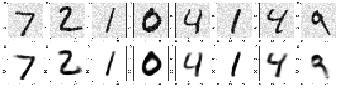
 source
Auto encoders were entirely new to me. I was glad I chose the task “Build a simple Auto-encoder model using tf.keras” because I learned a lot about them. They are probably the most interesting application of machine learning I have used so far.
I wrote a Colab tutorial detailing:
This tutorial was very well received by the mentors as well as Twitter:
During Christmas I wrote a blog post for the task: “Tutorial for Polynomial Regression.”. My blog post covers the basics of machine learning, the mathematical theory behind polynomial regression along with an implementation in Python. It also discusses feature selection and over/underfitting.
This post was featured on the front page of Hacker News for more than 18 hours getting more than 140 points. Hacker News users provided a lot of good feedback improving future content on this site. In total the post attracted over 6000 new users!
Contributing to open source projects was very exciting because I got to work with many smart people from all around the world including Googlers.
Some merged PRs I made during Code-In:
Before wrapping up this post I would like to take a moment to thank the awesome mentors, admins and the organizers of Code-In for this amazing event. I really learned a lot by taking part in it.
I would like to thank the TensorFlow mentors in particular for investing their time into helping us, the students, with valuable feedback and counselling. This event would not have been possible without you.
I’m happy I got a chance to work with these mentors:
If you are a mentor (thanks!) and your Twitter handle is missing, my DMs are open!
Y’all are awesome!
The deadline just passed. I guess I’ll have to wait patiently until the winners are announced on February 10th! I guess I won’t get to sleep very much…
Google just announced the winners and I’m super proud to be one of them! I can’t wait to visit California again :)
]]>Convenience is not the only motivation for this type of interaction, though. The combination of speech recognition and speech synthesis feels more personal than using a touch screen. On top of that, the option for verbal communication enables visually impaired people to interact with your app.
As you probably already know, Siri’s communication mechanism can be split up in two main components: speaking and listening. Speaking is formally known as “speech synthesis” whereas listening is often referred to as “speech recognition.” Although the tasks look very different in code, they have one thing in common: both are powered by machine learning.
Luckily, Apple’s speech synthesis and speech recognition APIs aren’t private — everyone has access to their cutting-edge technology. In this tutorial, you’ll build an app that uses those APIs to speak and listen to you.
]]>