Compressing images using Python
Compressing images is a neat way to shrink the size of an image while maintaining the resolution. In this tutorial we’re building an image compressor using Python, Numpy and Pillow. We’ll be using machine learning, the unsupervised K-means algorithm to be precise.
If you don’t have Numpy and Pillow installed, you can do so using the following command:
pip3 install pillow
pip3 install numpy
Start by importing the following libraries:
import os
import sys

from PIL import Image
import numpy as np
The K-means algorithm
K-means, as mentioned in the introduction, is an unsupervised machine learning algorithm. Simplified, the major difference between unsupervised and supervised machine learning algorithms is that supervised learning algorithms learn by example (labels are in the dataset), and unsupervised learning algorithms learn by trial and error; you label the data yourself.
I’ll be explaining how the algorithm works based on an example. In the illustration below there are two features, \(x_1\) and \(x_2\).
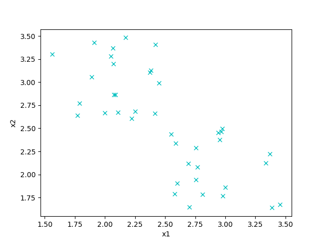
We want to assign each item to one out of two clusters. The most natural way to do this would be something like this:
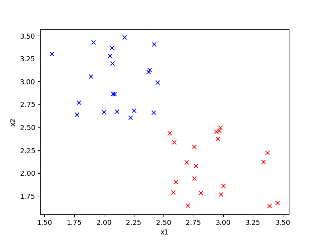
K-means is an algorithm to do exactly this. Note that \(K\) is the number of clusters we want to have, hence the name K means.
We start by randomly getting \(K\) training examples and in \(\mu\) so that the points are \(\mu_1, \mu_2, …, \mu_k\) and \(\mu \in \mathbb{R}^n\) where \(n\) is the number of features. At initialization, the points might be very close to one another, so we have to check if our result looks like how we want it to look because it might stuck be in a local optimum.
Then for a certain number of iterations, execute the following steps:
- For every training example, assign \(c^{(i)}\) to the closest centroid.
- For every centroid \(\mu_k\), set the location to be the average of examples assigned to it.
As the algorithm progresses, generally the centroids will move to the center of the clusters and the overall distance of the examples to the clusters gets smaller.
K-means for image compression
This technique can also be used for image compression. Each pixel of the image consists of three values, R(ed), B(lue) and G(reen). Those can be seen as the points on the grid, in 3D in case of RGB. The objective of image compression in this case is to reduce the number of colors by taking the average \(K\) colors that look closest to the original image. An image with fewer colors takes up less disk space, which is what we want.
Compressing the image can also be a preprocessing step to another algorithm. Reducing the size of the input data generally speeds up learning.
Implementing K-means
We start by implementing a function that creates initial points for the centroids. This function takes as input X, the training examples, and chooses \(K\) distinct points at random.
def initialize_K_centroids(X, K):
    """ Choose K points from X at random """
    m = len(X)
    return X[np.random.choice(m, K, replace=False), :]
Then we write a function to find the closest centroid for each training example. This is the first step of the algorithm. We take X and the centroids as input and return the the index of the closest centroid for every example in c, an m-dimensional vector.
def find_closest_centroids(X, centroids):
    m = len(X)
    c = np.zeros(m)
    for i in range(m):
        # Find distances
        distances = np.linalg.norm(X[i] - centroids, axis=1)

        # Assign closest cluster to c[i]
        c[i] = np.argmin(distances)

    return c
For the second step of the algorithm, we compute the distance of each example to ‘its’ centroid and take the average of distance for every centroid \(\mu_k\). Because we’re looping over the rows, we have to transpose the examples.
def compute_means(X, idx, K):
    _, n = X.shape
    centroids = np.zeros((K, n))
    for k in range(K):
        examples = X[np.where(idx == k)]
        mean = [np.mean(column) for column in examples.T]
        centroids[k] = mean
    return centroids
Finally, we got all the ingredients to complete the K-means algorithm. We set max_iter, the maximum number of iterations, to 10. Note that if the centroids aren’t moving anymore, we return the results because we cannot optimize any further.
def find_k_means(X, K, max_iters=10):
    centroids = initialize_K_centroids(X, K)
    previous_centroids = centroids
    for _ in range(max_iters):
        idx = find_closest_centroids(X, centroids)
        centroids = compute_means(X, idx, K)
        if (centroids == previous_centroids).all():
            # The centroids aren't moving anymore.
            return centroids
        else:
            previous_centroids = centroids

    return centroids, idx
Getting the image
In case you’ve never worked with Pillow before, don’t worry. The api is very easy.
We start by trying to open the image, which is defined as the first (and last) command line argument like so:
try:
    image_path = sys.argv[1]
    assert os.path.isfile(image_path)
except (IndexError, AssertionError):
    print('Please specify an image')
Pillow gives us an Image object, but our algorithm requires a NumPy array. So let’s define a little helper function to convert them. Notice how each value is divided by 255 to scale the pixels to 0…1 (a good ML practice).
def load_image(path):
    """ Load image from path. Return a numpy array """
    image = Image.open(path)
    return np.asarray(image) / 255
Here’s how to use that:
image = load_image(image_path)
w, h, d = image.shape
print('Image found with width: {}, height: {}, depth: {}'.format(w, h, d))
Then we get our feature matrix \(X\). We’re reshaping the image because each pixel has the same meaning (color), so they don’t have to be presented as a grid.
X = image.reshape((w * h, d))
K = 20 # the desired number of colors in the compressed image
Finally we can make use of our algorithm and get the \(K\) colors. These colors are chosen by the algorithm.
colors, _ = find_k_means(X, K, max_iters=20)
Because the indexes returned by the find_k_means function are 1 iteration behind the colors, we compute the indexes for the current colors. Each pixel has a value in \({0...K}\) corresponding, of course, to its color.
idx = find_closest_centroids(X, colors)
Once we have all the data required we reconstruct the image by substituting the color index with the color and resphaping the image back to its original dimensions. Then using the Pillow function Image.fromarray we convert the raw numbers back to an image. We also convert the indexes to integers because numpy only accepts those as indexes for matrices.
idx = np.array(idx, dtype=np.uint8)
X_reconstructed = np.array(colors[idx, :] * 255, dtype=np.uint8).reshape((w, h, d))
compressed_image = Image.fromarray(X_reconstructed)
Finally, we save the image back to the disk like so:
compressed_image.save('out.png')
Testing an image
This is the fun part, testing our program. You can choose any (png) image you want. I use this image by Valentin Pinisoara on Unsplash that I scaled down for speed purposes.
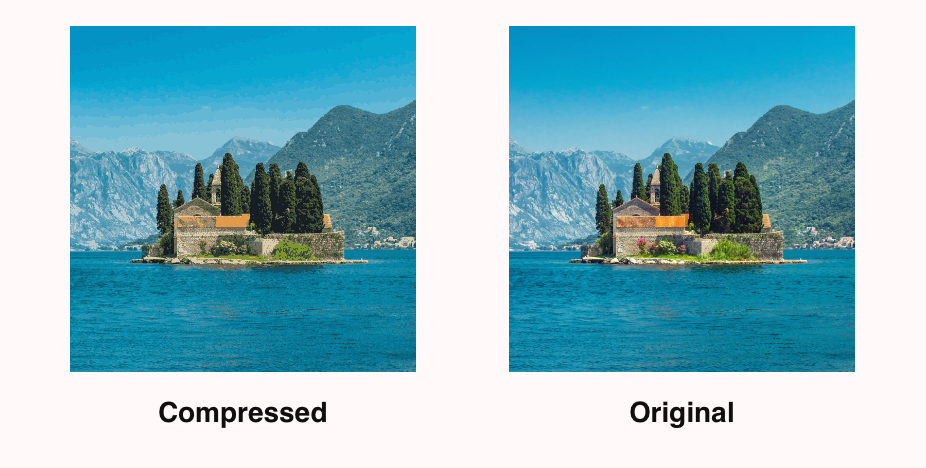
The file size was reduced by 71%, from 228kb to 65kb with \(K = 20\).
To get a better intuition for this algorith, you should try out different values for \(K\) and max_iter yourself.
Conclusion
As you’ve seen in this tutorial, it’s quite easy to reduce the file size of an image using unsupervised machine learning.
Check out the finished program on GitHub.
Thanks to Daniel Hess for reporting an error in this post.
Thanks for reading
I hope this post was useful to you. If you have any questions or comments, feel free to reach out on Twitter or email me directly at rick_wierenga [at] icloud [dot] com.