An Empirical Comparison of Optimizers for Machine Learning Models
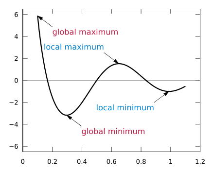
At every point in time during training, a neural network has a certain loss, or error, calculated using a cost function (also referred to as a loss function). This function indicates how ‘wrong’ the network (parameters) is based on the training or validation data. Optimally, the loss would be as low as possible. Unfortunately, cost functions are nonconvex — they don’t just have one minimum, but many, many local minima.
To minimize a neural network’s loss, an algorithm called backpropagation is used. Backpropagation calculates the derivative of the cost function with respect to the parameters in the neural network. In other words, it finds the “direction” in which to update the parameters so that the model will perform better. This “direction” is called a neural network’s gradient.
Before updating the model with the gradient, the gradient is multiplied by a learning rate. This yields the actual update on the neural network.. When the learning rate is too high, we might step over the minimum, meaning the model is not as good as it could have been.
But on the other hand, when the learning rate is too low, the optimization process is extremely slow. Another risk of a low learning rate is the fact that the state might end up in a bad local minimum. The model is at a suboptimal state as this point, but it could be much better.
This is where optimizers come in. Most optimizers calculate the learning rate automatically. Optimizers also apply the gradient to the neural network — they make the network learn. A good optimizer trains models fast, but it also prevents them from getting stuck in a local minimum.
Optimizers are the engine of machine learning — they make the computer learn.
Over the years, many optimizers have been introduced. In this post, I wanted to explore how they perform, comparatively.
Read full story on Heartbeat