Logistic Regression from Scratch in Python
ML from the Fundamentals (part 2)
Classification is one of the biggest problems machine learning explores. Where we used polynomial regression to predict values in a continuous output space, logistic regression is an algorithm for discrete regression, or classification, problems.
In the previous post I explained polynomial regression problems based on a task to predict the salary of a person given certain aspects of that person. I also discussed basic machine learning terminology. In this post I describe logistic regression and classification problems. By working through another example, predicting breast cancer, you will learn how to build your own classification model. I will also cover alternative metrics for measuring the accuracy of a machine learning model.
%pylab inline
The code is available in the corresponding GitHub repository for this series (leave a star :)). I encourage you to run the notebook alongside this post.
Classification
In a classification problem, the target values are called labels. Each label corresponds to a certain class such as “car”, “blue” or “malignant.” Each instance belongs to a certain class*, thus having a label. Both the labels and classes have to be unique, but more than one instance per class is allowed—it’s actually strongly encouraged. Usually each class’ label has an integer value starting at 0 and following classes get a label of 1, 2, 3, etc. This gives us the property that \(y^{(i)} \in \{0, 1, \ldots, K \}\) where $K$ is the number of classes.
With the terminology of the previous post, we could state that for binary classification \(y \in \{0, 1\}^m\) where \(0\) and \(1\) are labels. Further, in binary classification the instances belonging to the $0$-class are the “negatives”, often indicating the absence of a something, and $1$ are the “positives”. Another way to look at this is that for negatives there is a $0\%$ chance of something occurring where for positives there’s a $100\%$ chance. These percentages will, hopefully, be the output of a logistic regression model.
*If you wish to classify instances as not belonging to a certain class, you assign a “not classified” class.
The Dataset
The dataset we are working with today is the Breast Cancer Data Set [1]. For this dataset we have the following properties:
\[m = 669 \quad \quad n = 9\]To keep the blog post concise and focussed I added explanations in the notebook explaining how to load and clean the data with pandas.
Modelling
Much like the previous problem we need a way to map input values to output values. We will once again call this model \(h_\theta\).
Remember the model from polynomial regression:
\[h_\theta(x) = \theta^Tx\]We will make one small change to this model to work with classification.
Note that the model can output values much greater than $1$ and much smaller than $0$. This is unnatural and not desired—we would like to get values between $0$ and $1$ so we can interpret the output as probabilities. To achieve this we use the sigmoid function:
\[g(z) = \frac {1}{1+e^{-z}}\]Note: $g$ is a symbol for an activation function (more on that in future posts), not sigmoid.
While this function looks complicated, it’s easy to see why it’s used when you look at its graph:
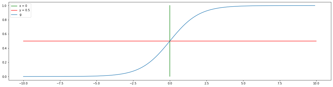
For values $x < 0$ we have that $g(x) < 0.5$ and for $x < 0$ we have $g(x) > 0.5$.
In Python you can just copy the formula over:
def g(z):
    """ sigmoid """
    return 1 / (1 + np.exp(-z))
As you can see, if we modify $h$ to be
\[h_\theta(x) = g(\theta^Tx)\]we have a model that outputs probabilities of an example $x$ belonging to the positive class, or $P(y = 1|x; \theta)$ in mathematical terms. For negative classes we have $P(y = 0|x; \theta) = 1 - P(y = 1|x; \theta)$.
During training we modify the values in $\theta$ to yield high values for $\theta^Tx$ when $x$ is a positive example, and vice versa.
def h(X, theta):
    return g(X @ theta)
Decision boundary
To make a final decision about which class a certain example $x$ belongs to we define a certain threshold. If $h$ exceeds that threshold we predict $1$, otherwise $0$. We most normally use $0.5$, we are more than $50%$ sure something will happen, but it depends on the context.*
If we are looking for labels, we have:
\[h_\theta(x) = g(\theta^Tx) > 0.5\]If you think about the feature space as an $n$-dimensional space, the decision boundary is a $n-1$-dimensional surface that divides the feature space in two. If you cross that surface the prediction about your class will change. The further you move away from the decision boundary the more certain you are about belonging to the class you’re in.
* More on that later in this post.
The loss function
Let’s look at mean squared error loss function again:
\[J(\theta) = \frac{1}{m}\displaystyle\sum_i^m (h_\theta(x^{(i)}) - y^{(i)})^2\]With this function you can optimize, minimize, the euclidean distance between a prediction and the target. While using this function would work with logistic regression, it turns out that it’s very hard to optimize with an optimization algorithm like gradient descent. The reason for this is because the loss function is very non-convex as a result of the nonlinearity $g$. In order words, we have more than one minimum and we’re not sure whether a certain minimum is the best fit for our model.
That’s the reason we use another loss function:
\[J(\theta) = \begin{cases} -\log(1 - h_\theta(x)) & \text{if } y = 0 \\ -\log(h_\theta(x)) & \text{if } y = 1 \end{cases}\]Let’s break that down by looking at a few examples. Suppose we have the label $y^{(i)}$ and the prediction $h_\theta(x^{(i)})$:
If $y^{(i)} = h_\theta(x^{(i)}) = 0$ we have a loss of $-\log(1 - h_\theta(x)) = -\log(1 - 0) = -\log1 = 0$
If $y^{(i)} = h_\theta(x^{(i)}) = 1$ we have a loss of $-\log(h_\theta(x)) = -\log1 = 0$
If $y^{(i)} = 0$ but $h_\theta(x^{(i)}) = 1$ we have a loss of $-\log(1 - h_\theta(x)) = -\log(1 - 1) = -\log0 = \infty$
If $y^{(i)} = 1$ but $h_\theta(x^{(i)}) = 1$ we have a loss of $-\log(h_\theta(x)) = -\log0 = \infty$
In general, as the model moves closer to the wrong prediction, the loss gets progressively higher. Let’s look at the loss of the sigmoid function $g$ with respect to $z$:
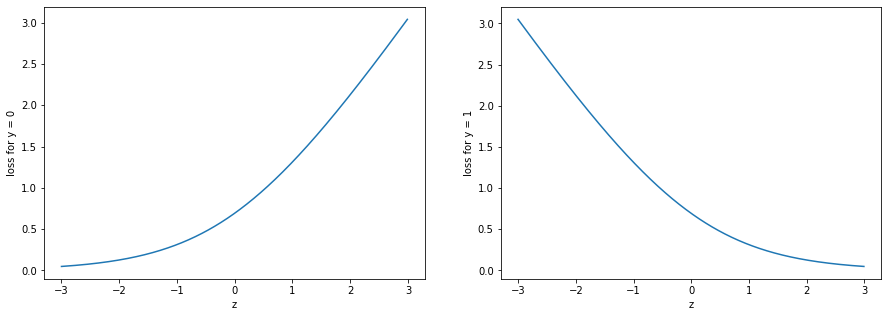
For $y = 0$, as $z$ approaches $-\infty$, $g(z)$ approaches $0$ so the loss approaches $0$ as well. For $y = 1$, as $z$ approaches $\infty$, $g(z)$ approaches $1$, so the loss approaches $0$.
Another way to understand this is that this loss function pushes the model to be very sure about its predictions. The model will always be penalized, even it if it predicts the correct class, except when it has 100% certainty. For example, let’s suppose the model is 51% sure ($h(x) = 0.51$) about an example belonging to class 1, thus predicting class 1, it will still have a loss of $- \log 0.51 \approx 0.67$.
Because we know that $y^{(i)} \in {0, 1}$, there’s a shorter way of writing this function:
\[J(\theta) = -\frac{1}{m}\begin{bmatrix}\displaystyle\sum_{i=1}^{m}y^{(i)}\log h_\theta(x^{(i)})+(1-y^{(i)})\log(1-h_\theta(x^{(i)}))\end{bmatrix}\]If $y^{(i)} = 1$ we have that $y^{(i)} = 1$, of course, so the first term will be multiplied by $1$ and $(1-y^{(i)})$ would be $1 - 1 = 0$ so the second part will be multiplied by $0$. The opposite is also true.
In Python:
def J(preds, y):
    return 1/m * (-y @ np.log(preds) - (1 - y) @ np.log(1 - preds))
Derivative
Just like polynomial regression, we will use the derivative of the loss function to calculate a gradient descent step.
The vectorized derivative for $J$ is given as:
\[\nabla J(X) = \frac{1}{m} X^T (X\theta - y)\]In Python:
def compute_gradient(theta, X, y):
  preds = h(X, theta)
  gradient = 1/m * X.T @ (preds - y)
  return gradient
Training
We will again use gradient descent as our optimization algorithm. For more information, refer to the first post in this series.
A basic training loop would look like this:
alpha = 0.1

for i in range(100):
  gradient = compute_gradient(theta, X, y)
  theta -= alpha * gradient
We will later update it to print out statistics about the performance of the model.
Measuring performance
One of the only ways we could measure performance of the polynomial regression model was through a loss function. Because classification problem are discrete, it opens up new possibilities to measure the performance, two of which I will be talking about now.
Accuracy
The first one is accuracy: the percentage of examples we correctly predicted the class for.
Implementing this in Python is very easy if we count the number of instances we get correct and divide it by the total number of items. In mathematical terms, that’s equal to the average.
preds = h(X, theta)
((preds > 0.5) == y).mean()
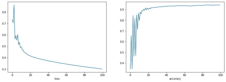
We can update the training loop to print out the accuracy and loss every 10 epochs:
hist = {'loss': [], 'acc': []}
alpha = 0.1

for i in range(100):
  gradient = compute_gradient(theta, X, y)
  theta -= alpha * gradient

  # loss
  preds = h(X, theta)
  loss = J(preds, y)
  hist['loss'].append(loss)

  # acc
  acc = ((h(X, theta) > .5) == y).mean()
  hist['acc'].append(acc)

  # print stats
  if i % 10 == 0: print(loss, acc)
This also keeps track of the loss and accuracy during training. If we plot the arrays we get the following graphs:
The F1 score
While accuracy might seem like a perfect metric to measure performance, it’s actually naive to believe that. For instance, suppose we had very few negatives in our dataset. Models that always predict $1$ will have a high accuracy while they are not actually very performant. So instead a better measure would be the F1 score: a scalar indicating model performance.
To understand it, let’s first look at the following table:
| label: 1 | label: 0 | |
|---|---|---|
| prediction: 0 | false negative | true negative |
| prediction: 1 | true positive | false positive |
The precision of a model is defined as:
\[p = \text{precision} = \frac{\text{True positives}}{\text{True positives}+\text{False positives}}\]def precision(preds, labels):
tp = ((preds == 1) == (y == 1)).sum()
fp = ((preds == 1) == (y == 0)).sum()
return tp / (tp + fp)
The recall of a model is defined as:
\[r = \text{recall} = \frac{\text{True positives}}{\text{True positives}+\text{False negatives}}\]def recall(preds, labels):
tp = ((preds == 1) == (y == 1)).sum()
fn = ((preds == 0) == (y == 1)).sum()
return tp / (tp + fn)
“$p$ is the number of correct positive results divided by the number of all positive results returned by the classifier, and $r$ is the number of correct positive results divided by the number of all relevant samples (all samples that should have been identified as positive)” source: Wikipedia
The F1 score is defined as the harmonic mean of the precision and recall:
\[F_{1}=\left({\frac {2}{\mathrm {recall} ^{-1}+\mathrm {precision} ^{-1}}}\right)=2\cdot {\frac {\mathrm {precision} \cdot \mathrm {recall} }{\mathrm {precision} +\mathrm {recall} }}\]def f1(preds, labels):
return 2 * (precision(preds, labels) * recall(preds, labels)) / (precision(preds, labels) + recall(preds, labels))
The optimal value is $1$, where we have perfect precision and recall. The worst value is, as you might expect, $0$.
Optimizing model performance
Back to our goal of classifying breast cancer in patients given certain statistics about the patient. Our model has quite a low recall of $0.5$. This means that our model has many false negatives: it did not predict cancer was present, while actually the patient did have cancer. Given our so-called domain knowledge, we might try to optimize for recall instead of accuracy: we would rather predict too many patients have cancer than too few.
Let’s make a plot of how the recall changes as we update the threshold:
recalls = []
for p in range(100):
    preds = (h(X, theta) > p)
    r = recall(preds, y)
    recalls.append(r)
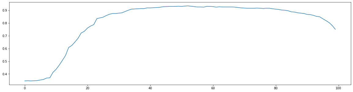
While our recall is already quite good, we can do a little better if we choose a threshold of $52\%$ as opposed to $50\%$.
Classification vs Regression
One could argue that the problem in the previous post could be regarded as a classification problem where the income is a label. This is a very valid argument, and we could build a classification model with no modifications to the dataset. However, given the context it is more natural to solve that problems with a regression model: salary is a continuous variable (continuous enough, that is). For breast cancer, deciding what kind of model to build is easy too: patients do not have “degrees of cancer.”
What’s next?
This was the second post of the “ML from the Fundamentals” series. In a future post I will be discussing neural networks: a more sophisticated solution for classification problems. We will also look at unsupervised learning (without targets). Be sure to follow me on Twitter so you stay up to date with the series. I’m @rickwierenga.
Sources
[1] Dheeru Dua en Casey Graff. UCI Machine Learning Repository. 2017. url: http://archive.ics.uci.edu/ml.
Thanks for reading
I hope this post was useful to you. If you have any questions or comments, feel free to reach out on Twitter or email me directly at rick_wierenga [at] icloud [dot] com.