Softmax Regression from Scratch in Python
ML from the Fundamentals (part 3)
Last time we looked at classification problems and how to classify breast cancer with logistic regression, a binary classification problem. In this post we will consider another type of classification: multiclass classification. In particular, I will cover one hot encoding, the softmax activation function and negative log likelihood.
Revisiting classification
Recall from the previous post that classification is discrete regression. The target $y^{(i)}$ can take on values from a discrete and finite set. In binary classification we only considered sets of size $2$, but classification can be extended beyond that. Let’s look at the complete picture where $y^{(i)} \in {0, 1, \ldots K}$.
The model we build for logistic regression could be intuitively understood by looking at the decision boundary. By forcing the model to predict values as distant from the decision boundary as possible through the logistic loss function, we were able to build theoretically very stable models. The model outputted probabilities for each instance belonging to the positive class.
However, in multiclass classification it’s hard to think about a decision boundary splitting the feature space in more than 2 parts. In fact, such a plane does not even exist. Furthermore, the log loss function does not work with more than two classes because it depends on the fact that if an instance belongs to one class, it does not belong to the other. So we need something else.
Let’s look at where we are thus far. A schematic of polynomial regression:

A corresponding diagram for logistic regression:

In this post we will build another model, which is very similar to logistic regression. The key difference in the hypothesis function is that we use $\sigma$ instead of sigmoid, $g$:

One hot encoding
As I just mentioned, we can’t measure distances over a single “class dimension” (by which I mean the probability of an instance belonging to the positive class). Instead, for multiclass classification we think about each class as a separate channel, or dimension if you will. All of these channels are accumulated in an output vector, $\hat{y} \in \mathbb{R}^K$.
Let’s take a look at what such a vector would look like. For convenience, we define a function $T(y): \mathbb{R} \rightarrow \mathbb{R}^K$ which maps labels from their integer representation (in $0, 1, \ldots k$) to a one hot encoded representation. This function takes into account the total number of classes, $3$ in this case.
\[T(0) = \begin{bmatrix}1 \\ 0 \\ 0 \end{bmatrix} \quad T(1) = \begin{bmatrix}0 \\ 1 \\ 0 \end{bmatrix}\]The instance in class $0$ has a $100\%$ chance of belonging to $1$, and a $0\%$ chance for all other classes. We would like $h$ to yield similar values.
In Python $T$ could be implemented as follows:
def T(y, K):
  """ one hot encoding """
  one_hot = np.zeros((len(y), K))
  one_hot[np.arange(len(y)), y] = 1
  return one_hot
If you don’t yet see why this would be useful yet, hang on.
Building the model: the softmax function
Up until now $x \cdot \theta$ has always had a scalar output, an output in one dimension. However, in this case the resulting value will be a vector where each row corresponds to a certain class, as we have just seen. While this could be achieved by initializing $\theta$ as an $n \times K$ dimensional matrix, which we will also do, the dot product would be of little meaning.
That’s the reason we define another activation function, $\sigma$. As you may remember from last post, $g$ is the general symbol for activation functions. But as you will learn in the neural networks post (stay tuned) the softmax activation function is a bit of an outlier compared to the other ones. So we use $\sigma$.
For $z\in\mathbb{R}^k$, $\sigma$ is defined as
\[\sigma(z) = \frac{\exp(z_i)}{\sum_{j=1}^k \exp(z_j)}\]which gives
\[p(y = i | x; \theta) = \frac{\exp(\theta_j^Tx)}{\sum_{j=1}^k \exp(\theta_j^Tx)}\]where $\theta_j \in \mathbb{R}^m$ is the vector of weights corresponding to class $i$. $p$ is the probability. For more details on why that is, refer to this document, section 9.3.
The hypothesis function $h$ yields a vector $\hat{y}$ where each row is the probability of the input $x$ belonging to a class. For $K = 3$ we have
\[h_\theta(x) = \sigma(X \cdot \theta) = \begin{bmatrix}p(y = 0 | x; \theta) \\ p(y = 1 | x; \theta) \\ p(y = 2 | x; \theta)\end{bmatrix} = \begin{bmatrix} \frac{\exp(\theta_0^Tx)}{\sum_{j=1}^k \exp(\theta_j^Tx)} \\ \frac{\exp(\theta_1^Tx)}{\sum_{j=1}^k \exp(\theta_j^Tx)} \\ \frac{\exp(\theta_2^Tx)}{\sum_{j=1}^k \exp(\theta_j^Tx)} \end{bmatrix}\]See how $T$ fits into the picture?
To get a final class prediction, we don’t check if the number exceeds a certain threshold ($0.5$ in the last post), but we take the channel with the highest probability. In mathematical terms:
\[\text{class} = \arg\max \hat{y}\]One thing I would like to point out here is that
\[\displaystyle\sum_{j=1}^k h_\theta(x)_j = 1\]This is obvious because the sum of numerators in $h$ is equal to the denominator, by definition.Intuitively, the model is $100\%$ sure each instance belongs to one of the predefined classes. Furthermore, because $\exp$ is, of course, an exponential function, large elements in $\theta^Tx$ will be “intensified” by $\sigma$ to get a higher probability, also relatively speaking.
A vectorized python implementation:
def softmax(z):
    return np.exp(z) / np.sum(np.exp(z))
Numerical stability
When implementing softmax, $\sum_{j=1}^k \exp(\theta_j^Tx)$ may be very high which leads to numerically unstable programs. To avoid this problem, we normalize each value $\theta_j^Tx$ by subtracting the largest value.
The implementation now becomes
def softmax(z):
    z -= np.max(z)
    return np.exp(z) / np.sum(np.exp(z))
This normalization step has no further impact on the outcomes.
The hypothesis
For the sake of completeness, here is the final implementation for the hypothesis function:
def h(X, theta):
    return softmax(X @ theta)
Negative log likelihood
The loss function is used to measure how bad our model is. Thus far, that meant the distance of a prediction to the target value because we have only looked at 1-dimensional output spaces. In multidimensional output spaces, we need another way to measure badness.
Negative log likelihood is yet another loss function suitable for these kinds of measurements. It is defined as:
\[J(\theta) = -\displaystyle\sum_{i = 1}^m \log p(y^{(i)}|x^{(i)};\theta)\]When I first encountered this function it was extremely confusing to me. But it turns out that the idea behind it is actually brilliant and even intuitive.
Let’s first look at the plot of the negative log likelihood for some arbitrary probabilities.
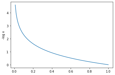
As the probability increases, the loss decreases. And because we only take the negative log likelihood of the current class, $y^{(i)}$ in the formula, into account, this looks like a nice property. Moreover, when we maximize the probability for the correct class, we automatically decrease the probabilities for other classes because the sum is always equal to $1$. This is an implicit side effect which might not be obvious at first.
We always want to get the loss as low as possible. The negative log likelihood is multiplied by $-1$, which means that you could also look at it as maximizing the log likelihood:
\[\displaystyle\sum_{i = 1}^m \log p(y^{(i)}|x^{(i)};\theta)\]Because all machine learning optimizers are designed for minimization instead of maximization, we use negative log likelihood instead of just the log likelihood.
Finally, here is a vectorized Python implementation:
def J(preds, y):
    return np.sum(- np.log(preds[np.arange(m), y]))
preds[np.arange(m), y] indixes all values of preds for each class of y, discarding the other probabilities.
Conclusion
If you would like to play around with the concepts I introduced yourself, I recommend you check out the corresponding notebook.
You now have all the necessary knowledge to learn about neural networks, the topic of next week’s post.
Thanks for reading
I hope this post was useful to you. If you have any questions or comments, feel free to reach out on Twitter or email me directly at rick_wierenga [at] icloud [dot] com.